ZO-1 mesh to force network¶

First, we import some general classes

[1]:

import pandas as pd
import seaborn as sns
import numpy as np
import pickle
import os
import sys
import pylab
import matplotlib.pyplot as plt

Then, DLITE classes

[2]:

from DLITE.cell_describe import node, edge, cell, colony
from DLITE.ManualTracingMultiple import ManualTracingMultiple
from DLITE.SurfaceEvolver import SurfaceEvolver
from DLITE.PlottingFunctions import PlottingFunctions

The main class we will be using here is the ManualTracingMultiple class

ManualTracingMultiple can read txt files of the form (name_first + number + name_end).

For example, name_first = ‘MAX_20170123_I01_003-Scene-4-P4-split_T’, number = 1, name_end = ‘.ome.txt’ is a txt file with the name ‘MAX_20170123_I01_003-Scene-4-P4-split_T1.ome.txt’.

Here, we have 30 timepoints so we define number as an integer from 0 to 29.

[3]:

os.chdir(r'../Notebooks/data/ZO-1_data/Time-series_1')
timepoints = [int(i) for i in np.linspace(0, 29, 30)]

Let’s instantiate the class

[4]:

ManualTracingMultipleInstance = ManualTracingMultiple(timepoints, name_first = 'MAX_20170123_I01_003-Scene-4-P4-split_T',
                                                           name_last = '.ome.txt', type=None)

Now, we can compute tensions! Here we’ll specify the solver as ‘CellFIT’

[5]:

colonies = ManualTracingMultipleInstance.main_computation_based_on_prev(timepoints, colonies = None, index = None,
                                          old_dictionary = None, solver = 'CellFIT', maxiter = 60*1000)

File 0 used a Cutoff value ------> 14

/Users/ritvikvasan/Documents/repos/DLITE/DLITE/cell_describe.py:908: LinAlgWarning: Ill-conditioned matrix (rcond=1.30265e-18): result may not be accurate.
  x = linalg.solve(r2, y)  # Solve Rx=y

Solver is CellFIT
First colony {'0': <DLITE.cell_describe.colony object at 0x11c84f6a0>}
File 1 used a Cutoff value ------> 14
node a = node b, possible topological change

/Users/ritvikvasan/Documents/repos/DLITE/DLITE/cell_describe.py:908: LinAlgWarning: Ill-conditioned matrix (rcond=3.6658e-20): result may not be accurate.
  x = linalg.solve(r2, y)  # Solve Rx=y

Next colony number 1
File 2 used a Cutoff value ------> 14

/Users/ritvikvasan/Documents/repos/DLITE/DLITE/cell_describe.py:908: LinAlgWarning: Ill-conditioned matrix (rcond=9.92725e-19): result may not be accurate.
  x = linalg.solve(r2, y)  # Solve Rx=y

Next colony number 2
File 3 used a Cutoff value ------> 14

/Users/ritvikvasan/Documents/repos/DLITE/DLITE/cell_describe.py:908: LinAlgWarning: Ill-conditioned matrix (rcond=2.85955e-18): result may not be accurate.
  x = linalg.solve(r2, y)  # Solve Rx=y

Next colony number 3
File 4 used a Cutoff value ------> 20
node a = node b, possible topological change
Next colony number 4
File 5 used a Cutoff value ------> 14
Next colony number 5
File 6 used a Cutoff value ------> 14
Next colony number 6
File 7 used a Cutoff value ------> 14
Next colony number 7
File 8 used a Cutoff value ------> 17
Next colony number 8
File 9 used a Cutoff value ------> 17
Next colony number 9
File 10 used a Cutoff value ------> 14
Next colony number 10
File 11 used a Cutoff value ------> 14
Next colony number 11
File 12 used a Cutoff value ------> 12
Next colony number 12
File 13 used a Cutoff value ------> 14

/Users/ritvikvasan/Documents/repos/DLITE/DLITE/cell_describe.py:908: LinAlgWarning: Ill-conditioned matrix (rcond=1.80949e-18): result may not be accurate.
  x = linalg.solve(r2, y)  # Solve Rx=y

Next colony number 13
File 14 used a Cutoff value ------> 16
Next colony number 14
File 15 used a Cutoff value ------> 16
Next colony number 15
File 16 used a Cutoff value ------> 17
Next colony number 16
File 17 used a Cutoff value ------> 14
Next colony number 17
File 18 used a Cutoff value ------> 16
Next colony number 18
File 19 used a Cutoff value ------> 16
Next colony number 19
File 20 used a Cutoff value ------> 16
node a = node b, possible topological change
Next colony number 20
File 21 used a Cutoff value ------> 12
Next colony number 21
File 22 used a Cutoff value ------> 16
Next colony number 22
File 23 used a Cutoff value ------> 16
Next colony number 23
File 24 used a Cutoff value ------> 16
Next colony number 24
File 25 used a Cutoff value ------> 16
Next colony number 25
File 26 used a Cutoff value ------> 16
Next colony number 26
File 27 used a Cutoff value ------> 16
Next colony number 27
File 28 used a Cutoff value ------> 16
node a = node b, possible topological change
Next colony number 28
File 29 used a Cutoff value ------> 16
Next colony number 29

This will give us 30 colony classes (for each time point)

[7]:

colonies

[7]:

{'0': <DLITE.cell_describe.colony at 0x11c84f6a0>,
 '1': <DLITE.cell_describe.colony at 0x10a737da0>,
 '2': <DLITE.cell_describe.colony at 0x120948b38>,
 '3': <DLITE.cell_describe.colony at 0x120995780>,
 '4': <DLITE.cell_describe.colony at 0x1209da390>,
 '5': <DLITE.cell_describe.colony at 0x120a0ef28>,
 '6': <DLITE.cell_describe.colony at 0x120a57d30>,
 '7': <DLITE.cell_describe.colony at 0x120a7ccf8>,
 '8': <DLITE.cell_describe.colony at 0x11c89dcc0>,
 '9': <DLITE.cell_describe.colony at 0x120af3cf8>,
 '10': <DLITE.cell_describe.colony at 0x120b8bc88>,
 '11': <DLITE.cell_describe.colony at 0x120bd8b38>,
 '12': <DLITE.cell_describe.colony at 0x120c1e828>,
 '13': <DLITE.cell_describe.colony at 0x120c67588>,
 '14': <DLITE.cell_describe.colony at 0x120c882b0>,
 '15': <DLITE.cell_describe.colony at 0x120c81fd0>,
 '16': <DLITE.cell_describe.colony at 0x120d16d30>,
 '17': <DLITE.cell_describe.colony at 0x120d34ac8>,
 '18': <DLITE.cell_describe.colony at 0x120dc67b8>,
 '19': <DLITE.cell_describe.colony at 0x120e0e550>,
 '20': <DLITE.cell_describe.colony at 0x120e562e8>,
 '21': <DLITE.cell_describe.colony at 0x120e77f98>,
 '22': <DLITE.cell_describe.colony at 0x120eb1d68>,
 '23': <DLITE.cell_describe.colony at 0x120efca90>,
 '24': <DLITE.cell_describe.colony at 0x120f2df60>,
 '25': <DLITE.cell_describe.colony at 0x120d94da0>,
 '26': <DLITE.cell_describe.colony at 0x120f83c50>,
 '27': <DLITE.cell_describe.colony at 0x120fcea90>,
 '28': <DLITE.cell_describe.colony at 0x1210158d0>,
 '29': <DLITE.cell_describe.colony at 0x1210cb710>}

Now, we need to do post processing

This is the same as before. We store all the information in 3 dataframes and we do this using the PlottingFunctions class in DLITE

[8]:

PlottingFunctionsInstance = PlottingFunctions()

[9]:

# We first find labels of edges that are present in all the colonies

common_edge_labels = PlottingFunctionsInstance.get_repeat_edge(colonies)
common_cell_labels = PlottingFunctionsInstance.get_repeat_cell(colonies)

[10]:

# Make the dataframes


edges_dataframe, cells_dataframe = PlottingFunctionsInstance.seaborn_plot(None, colonies,
                                                                                  common_edge_labels,
                                                                                  common_cell_labels,
                                                                                  ground_truth = None)
nodes_dataframe = PlottingFunctionsInstance.seaborn_nodes_dataframe(colonies, None)
tensor_dataframe = PlottingFunctionsInstance.seaborn_cells_dataframe_tensor(colonies)

/Users/ritvikvasan/Documents/repos/DLITE/DLITE/PlottingFunctions.py:1352: RuntimeWarning: invalid value encountered in double_scalars
  cell_data['Pressures'].append([2*((c.pressure - min_pres) / float(max_pres - min_pres)) - 1 for c in v.cells if c.label == cell_lab][0])
/Users/ritvikvasan/Documents/repos/DLITE/DLITE/PlottingFunctions.py:1360: RuntimeWarning: invalid value encountered in double_scalars
  - min_pres) / float(max_pres - min_pres))

Once we have the dataframes, we can start plotting the results!

Here’s a heatmap of dynamic edge tensions

[11]:

tension_table = edges_dataframe.pivot_table(
        values='Local_normalized_tensions',
        index=['Edge_Labels'],
        columns='Time')

[12]:

sns.set_context("paper", font_scale=3)
%matplotlib inline
fig, ax = plt.subplots(1, 1, figsize = (5,10),sharey=True)
sns.heatmap(tension_table, ax=ax,
            vmin=0, vmax=3,cmap = 'jet')

[12]:

<matplotlib.axes._subplots.AxesSubplot at 0x1211be438>

../_images/ZO-1_data_ZO-1_Mesh_To_Force_Network_22_1.png

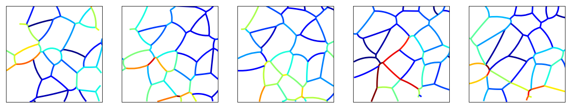
Here’s some colony colormaps at time points 0, 5, 10, 15 and 20

[13]:

# Plot
import pylab
import matplotlib.pyplot as plt


sns.set(style="white")
sns.set_context("paper", font_scale = 2.5)

total = 5
fig, axn = plt.subplots(1, total, figsize = (20,20),sharey=True)
nums= [0,5,10,15,20]

for i, ax in enumerate(axn.flat):
    col = colonies[str(nums[i])]
    tensions = [e.tension for e in col.tot_edges]
    mean_ten = np.mean(tensions)
    tensions = [e/mean_ten for e in tensions]

    col.plot_tensions(ax, fig, tensions, min_x=0, max_x=1000, min_y=0, max_y=1000,
                      min_ten = 0, max_ten = 3, specify_color = 'jet',cbar = 'no', lw = 3)
    plt.setp(ax.get_yticklabels(), visible=False)
    plt.setp(ax.get_xticklabels(), visible=False)
    ax.set(xlim = [0,1000], ylim = [0,1000], aspect = 1)

../_images/ZO-1_data_ZO-1_Mesh_To_Force_Network_24_0.png

As before, movies are also possible using something like this

[12]:

sns.set(style="darkgrid")
sns.set_context("talk", font_scale=0.75)

fig, ax = plt.subplots(1,1, figsize = (6,4))

PlottingFunctionsInstance.plot_tensions(fig, ax, colonies,min_x=0, max_x=1000, min_y=0, max_y=1000,
                                            min_ten=0,max_ten=3, specify_aspect=None,specify_color='jet' ,
                                            type=None, lw = 2)